12 Must-Know Data Structures for Coding Interviews

Cracking a coding interview isn’t just about writing code—it’s about solving problems efficiently. And to do that, you need to think in terms of data structures.

The right data structure can mean the difference between an algorithm that runs in milliseconds and one that times out completely.

While there are many data structures in computer science, some appear in coding interviews far more frequently than others.

In this article, we’ll go over 12 essential data structures that you must know for coding interviews.

---

1. Array

An array is a contiguous block of memory that stores elements of the same data type. Each element is identified by an index, allowing constant-time access (O(1)).

An array is stored sequentially in memory. Given an index, the memory address is calculated as:

Address = Base Address + (Index × Size of each element)

This is why accessing an element by index is O(1)—the address is computed directly.

When to Use an Array?

• You need fast access to elements using an index (O(1)).

• The number of elements is fixed or changes infrequently.

• You want a simple and efficient way to store sequential data.

• Memory locality is important (since arrays are contiguous, CPU caching is optimized).

Time & Space Complexities

Space Complexity: O(n) (since arrays store n elements)

Other Important Details

1. Fixed Size – In Java, arrays have a fixed size once created. You cannot dynamically resize an array.

2. Resizing Overhead – If you need resizing, use ArrayList, which internally doubles the size when capacity is exceeded.

---

2. Matrix

A matrix is essentially a two-dimensional array, where data is arranged in rows and columns.

A matrix is stored in memory row-wise in most programming languages (including Java). Each element is accessed using matrix[row][column].

When to Use a Matrix?

• When working with grid-based problems (chessboard, Sudoku, word search).

• For mathematical operations, like linear algebra, transformations, or machine learning.

• For graph representations using adjacency matrices.

• In image processing (storing pixels as a 2D array).

• In dynamic programming (e.g., dp[][] for problems like LCS, Knapsack).

Time & Space Complexities

Space Complexity: O(n × m) (since we store n × m elements).

---

3. Linked List

A linked list is a linear data structure where elements (nodes) are connected via pointers instead of being stored in a contiguous memory block. Each node consists of:

1. Data – The actual value stored in the node.

2. Pointer (next) – A reference to the next node in the list.

Unlike arrays, linked lists don’t require pre-allocated memory and allow dynamic resizing, making them efficient for insertions and deletions.

How is a Linked List Represented

class Node {
    int data;
    Node next;

    public Node(int data) {
        this.data = data;
        this.next = null;
    }
}

Types of Linked Lists

1. Singly Linked List (SLL)

• Each node has a next pointer to the next node.

• One-directional traversal.

2. Doubly Linked List (DLL)

• Each node has next and prev pointers.

• Allows bi-directional traversal.

3. Circular Linked List (CLL)

• The last node points back to the head, forming a loop.

When to Use a Linked List?

• When insertions/deletions are frequent (since they are O(1) at the head or tail).

• When memory fragmentation is a concern (as nodes are dynamically allocated).

• When dynamic resizing is required.

• When building LRU caches, stacks, and queues.

Time & Space Complexities

---

4. HashMap

A HashMap is a key-value pair data structure that provides fast lookups, insertions, and deletions using hashing. Unlike arrays or linked lists, HashMaps allow constant-time (O(1)) operations on average, making them extremely efficient for many applications.

How is a HashMap Represented?

A HashMap is internally implemented using an array of linked lists (buckets). When a key-value pair is inserted:

1. The key is hashed to generate an index.

2. The value is stored in the bucket corresponding to that index.

3. If multiple keys hash to the same index (collision), a linked list (or balanced BST) is used to store multiple values at that index.

Example:

Keys → Hash Function → Bucket Index
"John" → hash("John") → 2  →  [ ("John", 25) ]
"Mary" → hash("Mary") → 5  →  [ ("Mary", 30) ]
"Tom"  → hash("Tom")  → 2  →  [ ("John", 25), ("Tom", 40) ] (collision)

If two keys hash to the same bucket, chaining (linked list or tree) resolves the conflict.

When to Use a HashMap?

• When fast lookups (O(1)) are required.

• When frequent insertions and deletions are needed.

• When implementing caches, frequency counters, and indexing.

• When storing mappings between two datasets, e.g., usernames to user IDs.

Time & Space Complexities

---

5. Stack

A stack is a linear data structure that follows the Last In, First Out (LIFO) principle. This means the last element added is the first one to be removed—like a stack of plates in a cafeteria.

Example:

Push(10) → [10]
Push(20) → [10, 20]
Push(30) → [10, 20, 30]
Pop()    → [10, 20]  (30 is removed)
Peek()   → 20  (Top element)

Stacks support push, pop, and peek operations.

How is a Stack Represented?

Stacks can be implemented using:

1. Arrays (Fixed size, faster access)

2. Linked Lists (Dynamic size, extra memory overhead)

When to Use a Stack?

• When Last-In-First-Out (LIFO) order is required.

• When handling recursive function calls.

• For undo/redo functionality in text editors.

• When parsing expressions (e.g., checking balanced parentheses).

Time & Space Complexities

Array-based stacks have fixed size but are faster. Linked list-based stacks are dynamically resizable but use extra memory for pointers.

---

6. Queue

A queue is a linear data structure that follows the First In, First Out (FIFO) principle. The element added first is removed first, just like a real-world queue at a ticket counter.

Example:

Enqueue(5) → [5]
Enqueue(2) → [5, 2]
Enqueue(9) → [5, 2, 9]
Enqueue(4) → [5, 2, 9, 4]
Dequeue()  → [2, 9, 4]  (5 is removed)
Front()    → 2  (Next to be removed)

Queues support enqueue (insert), dequeue (remove), front (peek), and isEmpty operations.

How is a Queue Represented?

Queues can be implemented using:

1. Arrays (Fixed size, efficient indexing)

2. Linked Lists (Dynamic size, memory overhead)

When to Use a Queue?

• When FIFO (First-In-First-Out) ordering is required.

• When processing tasks in order (e.g., scheduling, messaging).

• When implementing BFS (Breadth-First Search) in graphs.

• When handling real-time requests, like task scheduling in OS.

Time & Space Complexities

---

7. Tree

A tree is a hierarchical data structure that consists of nodes connected by edges. Unlike arrays, linked lists, stacks, or queues (which are linear structures), trees are non-linear and provide fast search, insert, and delete operations in structured data.

Each tree consists of:

• Root – The topmost node.

• Parent & Child Nodes – A node that has child nodes is called a parent.

• Leaf Nodes – Nodes with no children.

• Height – The longest path from the root to a leaf.

The most popular type of tree is binary tree where each node has at most two children.

How is a Tree Represented?

Trees are implemented using nodes and references:

class TreeNode {
    int data;
    TreeNode left, right;

    public TreeNode(int data) {
        this.data = data;
        this.left = this.right = null;
    }
}

Tree Traversals

• Inorder: Left → Root → Right

• Preorder: Root → Left → Right

• Postorder: Left → Right → Root

• Level Order: Level by level

---

8. Binary Search Tree (BST)

A BST is a special type of binary tree where each node follows the BST property:

• The left subtree contains values smaller than the root.

• The right subtree contains values greater than the root.

• No duplicate values are allowed.

BSTs when balanced, provide efficient searching, insertion, and deletion (O(log n) on average), making them ideal for sorted data retrieval.

When to Use a BST?

• When you need fast search, insert, and delete operations (O(log n) average case).

• When you require sorted data retrieval (Inorder Traversal gives sorted order).

• When implementing symbol tables, dictionaries, and range queries.

• When handling dynamic data that needs frequent insertions/deletions.

Time & Space Complexities

If the BST degenerates into a linked list, operations become O(n).

Self-Balancing Trees (like AVL, Red-Black) keep operations at O(log n).

---

9. Heaps

A heap is a complete binary tree that satisfies the heap property:

• In a Min-Heap, the parent node is always smaller than its children.

• In a Max-Heap, the parent node is always greater than its children.

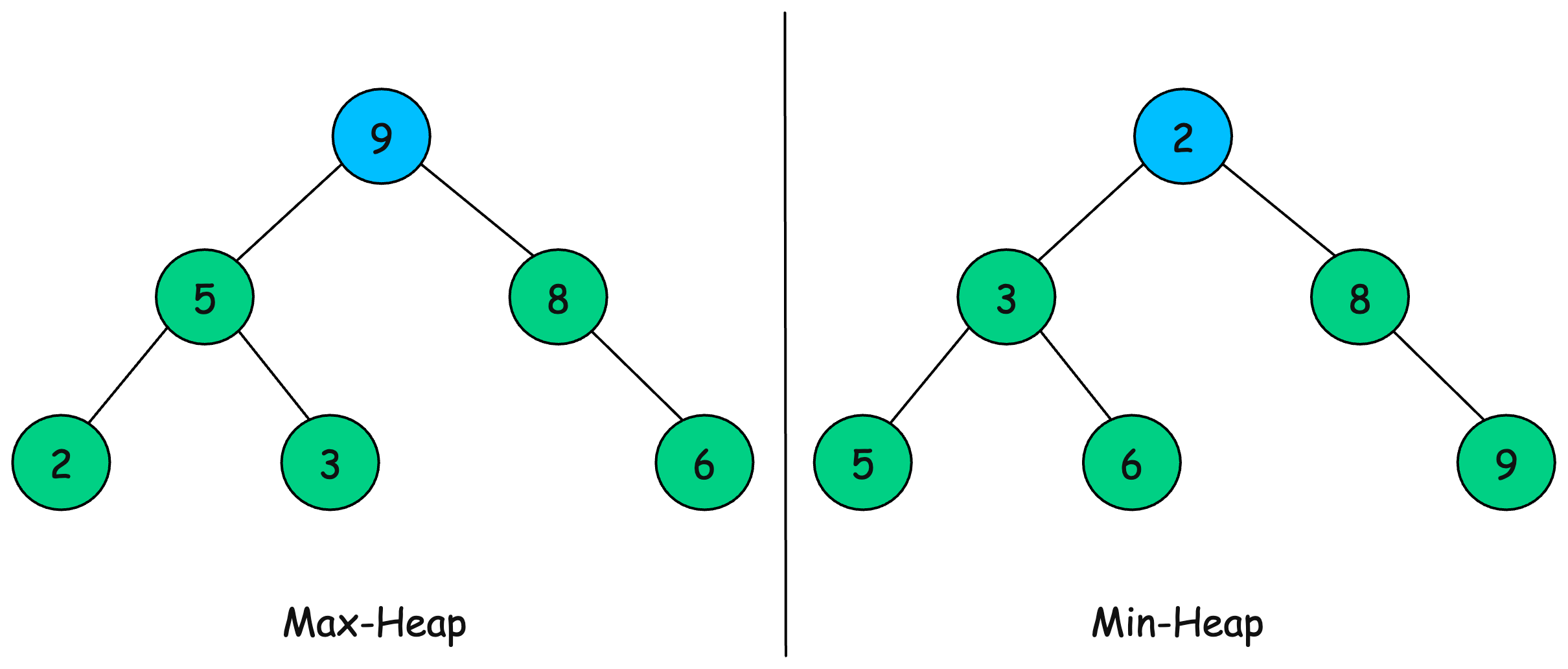
Unlike binary search trees (BSTs), heaps are optimized for fast retrieval of the minimum or maximum element.

How is a Heap Represented?

A heap is stored using a binary tree, but it's typically implemented using an array (to save space and make operations efficient).

For an element at index i:

• Left Child → 2 * i + 1

• Right Child → 2 * i + 2

• Parent → (i - 1) / 2

When to Use a Heap?

• When you need fast access to the smallest or largest element (O(1)).

• When implementing priority queues.

• When scheduling tasks based on priority (CPU scheduling, Dijkstra’s algorithm).

• When solving problems like Top K Elements, Median Finding, Heap Sort.

Time & Space Complexities

---

10. Trie

A Trie (also called a Prefix Tree) is a specialized tree structure used to store and search words efficiently. Unlike a binary tree, where each node contains a value, a Trie node represents a single character, and words are formed by linking nodes together.

Example:

Consider inserting the words: "ace", "ant", "cat", "pen" and "pet" into a Trie:

The main advantage of a Trie is fast prefix-based searching, making it ideal for applications like autocomplete, spell checkers, and IP routing.

How is a Trie Represented?

Each node contains:

• A HashMap/Array of child nodes (storing characters).

• A boolean flag (isEndOfWord) indicating the end of a word.

class TrieNode {
    TrieNode[] children = new TrieNode[26]; // Supports 'a' to 'z'
    boolean isEndOfWord;
}

When to Use a Trie?

• When fast prefix-based searching is needed (O(m), where m is word length).

• When implementing autocomplete suggestions.

• When handling dictionary-related problems (spell checkers, word games).

• When searching for words in large datasets efficiently.

Time & Space Complexities

---

11. Graph

A graph is a non-linear data structure consisting of nodes (vertices) and edges that connect them.

Graphs are used to model real-world relationships such as social networks, road maps, and the internet.

Types of Graphs

• Directed Graph (Digraph) – Edges have direction.

• Undirected Graph – Edges are bidirectional.

• Weighted Graph – Edges have weights.

• Unweighted Graph – All edges are equal.

• DAG (Directed Acyclic Graph) - Edges have direction but there is no cycle.

Graph Representation in Code

Graphs are implemented using:

1. Adjacency Matrix – 2D array

Each cell graph[i][j] = 1 means an edge exists between i and j.

class GraphMatrix {
    private int[][] adjMatrix;
    private int size;

    public GraphMatrix(int size) {
        this.size = size;
        adjMatrix = new int[size][size];
    }

    public void addEdge(int u, int v) {
        adjMatrix[u][v] = 1;
        adjMatrix[v][u] = 1; // For undirected graphs
    }

    public boolean isConnected(int u, int v) {
        return adjMatrix[u][v] == 1;
    }
}

Fast lookup O(1), but space inefficient O(V²).

2. Adjacency List – Array of lists

Each node stores a list of neighbors.

class GraphList {
    private Map<Integer, List<Integer>> adjList;

    public GraphList() {
        adjList = new HashMap<>();
    }

    public void addEdge(int u, int v) {
        adjList.computeIfAbsent(u, k -> new ArrayList<>()).add(v);
        adjList.computeIfAbsent(v, k -> new ArrayList<>()).add(u); // Undirected graph
    }

    public List<Integer> getNeighbors(int node) {
        return adjList.getOrDefault(node, new ArrayList<>());
    }
}

Efficient O(V + E) space, but slower O(V) lookup.

---

12. Union Find

Union-Find, also called Disjoint Set Union (DSU), is a data structure used to efficiently track and merge disjoint sets. It supports two main operations:

1. Find(x) → Determines the root representative (or parent) of a set containing x.

2. Union(x, y) → Merges the sets containing x and y.

Example:

Consider initially disjoint sets {1}, {2}, {3}, {4}, {5}, {6}

Performing union(1, 3), union(2, 4) and union(2, 5) gives:

• find(1) returns 1.

• find(4) returns 2 (as 4 is merged with 2).

How is Union-Find Represented?

Union-Find is implemented using:

1. An array (parent[]) where parent[i] points to the parent of node i.

2. Path Compression to speed up find(x).

3. Union by Rank to keep trees balanced.

class UnionFind {
    private int[] parent, rank;

    public UnionFind(int size) {
        parent = new int[size];
        rank = new int[size];
        for (int i = 0; i < size; i++) {
            parent[i] = i;  // Initially, each node is its own parent
            rank[i] = 1;    // Initial rank is 1
        }
    }

    public int find(int x) {
        if (parent[x] != x) {
            parent[x] = find(parent[x]); // Path compression
        }
        return parent[x];
    }

    public void union(int x, int y) {
        int rootX = find(x);
        int rootY = find(y);
        if (rootX == rootY) return;

        // Union by rank
        if (rank[rootX] > rank[rootY]) {
            parent[rootY] = rootX;
        } else if (rank[rootX] < rank[rootY]) {
            parent[rootX] = rootY;
        } else {
            parent[rootY] = rootX;
            rank[rootX]++;
        }
    }

    public boolean connected(int x, int y) {
        return find(x) == find(y);
    }
}

When to Use Union-Find?

• When checking connected components in a graph.

• When detecting cycles in an undirected graph.

• When performing dynamic connectivity queries.

• When implementing Kruskal’s Minimum Spanning Tree (MST) Algorithm.

Time & Space Complexities

α(n) is the inverse Ackermann function (nearly constant time).

---

Thank you for reading!

If you found it valuable, hit a like ❤️ and consider subscribing for more such content every week.

---

P.S. If you’re enjoying this newsletter and want to get even more value, consider becoming a paid subscriber.

As a paid subscriber, you'll receive an exclusive deep dive every Thursday, access to a structured system design resource, and other premium perks.

There are group discounts, gift options, and referral bonuses available.

---

Checkout my Youtube channel for more in-depth content.

Follow me on LinkedIn and X to stay updated.

Checkout my GitHub repositories for free interview preparation resources.

I hope you have a lovely day!

See you soon,

Ashish