Big-O Notation: Explained in 8 Minutes

Big O Notation is a way to measure how efficiently your code performs as the input size grows.

You’ve probably seen code that works perfectly on small inputs but slows down, crashes, or times out when the input becomes large.

Understanding Big O helps you avoid slow, inefficient solutions and write code that actually scales.

It’s also one of the most important topics in coding interviews.

You’ll almost always be asked to explain the time and space complexity of your solution and the more efficient your approach, the stronger your chances of passing the interview.

In this article, I’ll break down:

• What Big O Notation actually means

• The most common time complexities you’ll come across

• What is space complexity

• and rules to calculate Big O for any piece of code

---

I also made a 8 minutes video on Big-O notation. Check it out for more in-depth and visual explanation.

Subscribe for more such videos!

---

1. What is Big O?

So… what exactly is Big O Notation?

Big O is a mathematical way to describe how the performance of an algorithm changes as the size of the input grows.

It doesn’t tell you the exact time your code will take.

Instead, it gives you a high-level growth trend, how fast the number of operations increases relative to the input size.

For example: if your input doubles, does your algorithm take twice as long? Ten times as long? Or does it barely change at all?

Big O helps you answer those questions without even running the code so you can choose the most efficient algorithm for large inputs.

One important thing to note is that Big O is machine-independent.

It doesn’t matter whether your code runs on a fast laptop or a slow server, the growth pattern stays the same.

The key variable that drives BIG O is the input size (N). As N increases, Big O helps you predict whether the algorithm will still be efficient or become impractical.

---

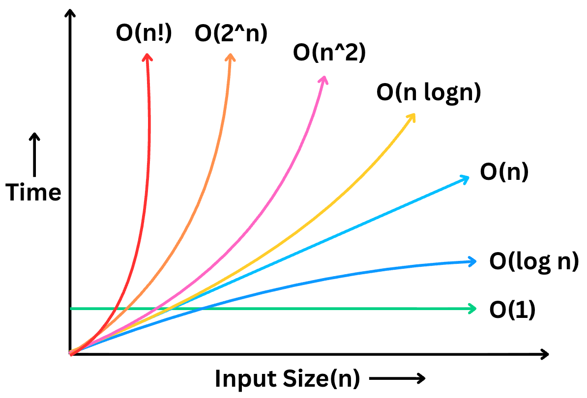
2. Common Run Time Complexities

Now that you understand what Big O Notation is, let’s go over the most common time complexities you’ll encounter.

Constant Time – O(1)

This is the fastest and most efficient time complexity.

An algorithm is O(1) if it performs a fixed number of operations meaning the execution time does not depend on the size of the input.

A classic example is accessing an element in an array by index.

int[] a = {10, 20, 30, 40}

int x = a[3];

System.out.println(x);

It doesn’t matter if the array has 10 elements…or 10 million, the time it takes to access an element stays exactly the same.

Logarithmic Time – O(log n)

An algorithm runs in O(log n) time when every step reduces the problem size by a constant factor (most often, by half).

This means the amount of work grows very slowly, even when the input becomes massive.

The most common example is Binary Search.

int binarySearch(int[] a, int target) {
    int lo = 0, hi = a.length - 1;
    
    while (lo <= hi) {
        int mid = lo + (hi - lo) / 2;
        if (a[mid] == target) 
          return mid;
        if (a[mid] < target) 
          lo = mid + 1;
        else 
          hi = mid - 1;
    }
    return -1;
}

Each step discards 50% of the remaining data.

To put that into perspective, here are the number of steps binary search takes for different input sizes.

• Input size = 8 → max 3 steps

• Input size = 1,000 → max 10 steps

• Input size = 1,000,000 → max 20 steps

• Input size = 1,000,000,000 → still just 30 steps!

Linear Time – O(n)

An algorithm is O(n) when its running time grows directly in proportion to the size of the input.

If the input doubles, the number of operations also doubles.

A simple example is finding the maximum value in an array:

int findMax(int[] array) {
    int max = array[0];
    for (int i = 1; i < array.length; i++) {
        if (array[i] > max) {
            max = array[i];
        }
    }
    return max;
}

• You start with some initial max

• Then you scan every element and compare it to the current max

• Each comparison is O(1), but you do it n times so the overall time complexity becomes O(n).

So with 10 elements, you do 10 comparisons. With 1 million elements, you do 1 million comparisons.

Any algorithm that visits every element exactly once is linear time.

Linearithmic Time – O(n log n)

Algorithms with O(n log n) time complexity combine two behaviors:

• A log n factor from repeatedly splitting the input

• An n factor from processing or merging the pieces

It’s often described as logarithmic splitting with linear merging.

The classic example is Merge Sort:

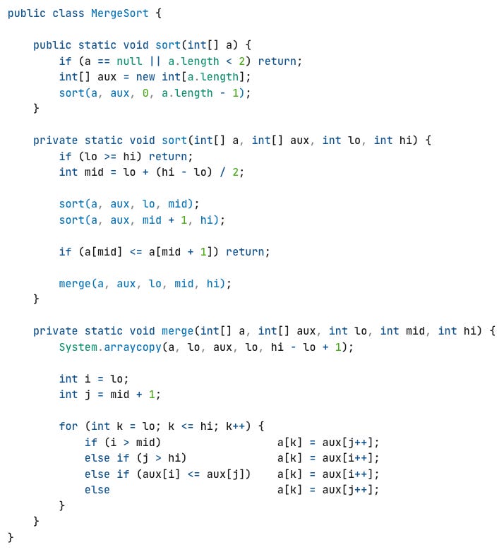
• First, it recursively splits the array in half over and over. That’s the log n part.

• Then, it merges the sorted halves back together and that takes n steps in total.

Multiply those together and you get O(n log n).

This complexity is slightly slower than linear time, but still very efficient and it’s the backbone of many fast sorting algorithms

Quadratic Time – O(n²)

In an O(n²) algorithm, the number of operations grows proportionally to the square of the input size. So if you have n elements, you perform roughly n × n operations.

This typically happens when you have nested loops, where for each element you iterate over all other elements.

public class NSquare {
    public int nsquare(int[] a) {
        int n = a.length;

        int pairSum = 0;

        for (int i = 0; i < n; i++) {
            for (int j = i + 1; j < n; j++) {
                pairSum += a[i] * a[j];
            }
        }

        return pairSum;
    }
}

Classic examples include simple sorting algorithms like:

• Bubble Sort

• Selection Sort

• Insertion Sort (worst case)

All of them compare or swap elements in nested loops, leading to O(n²) behavior.

These algorithms are fine for small inputs, but they become painfully slow as n grows:

For n = 1,000, you’re doing around 1 million operations. And if n = 10,000, you’re looking at 100 million operations.

In coding interviews and wherever performance matters, you’ll often want to avoid O(n²) and look for ways to bring it down to O(n log n) or better.

Exponential Time – O(2ⁿ)

Exponential time algorithms usually appear when we try to solve a problem by checking every possible combination often through brute force or backtracking.

Think of it as the opposite of binary search: Instead of eliminating half the work at each step, you are often doubling the work with each extra input element.

This happens in problems where each element can branch into multiple recursive calls.

A classic example is generating all subsets of a set (also called the power set):

• If the set has n elements, there are 2ⁿ possible subsets.

That means, just for 30 elements, you’re looking at over 1 billion possibilities. And for 40? Over 1 trillion.:

• n = 20 → ~1 million possibilities

• n = 30 → ~1 billion possibilities

• n = 40 → ~1 trillion possibilities

This kind of growth becomes unmanageable very quickly. Even a small increase in n makes the runtime explode.

But the good news is that many exponential-time problems can be optimized using techniques like memoization or dynamic programming

These techniques prevent us from recomputing the same subproblems, often reducing the time from O(2ⁿ) down to a much more practical polynomial time, which makes the solution usable in real-world scenarios.

In general, exponential algorithms are fine only for very small inputs. For anything larger, you must either optimize or rethink the approach.

Factorial Time – O(n!)

And finally… we’ve reached the most explosive time complexity of them all: Factorial Time, or O(n!)

This is what you get when an algorithm tries every possible arrangement of a set of n elements.

The number of possibilities grows faster than any other complexity we’ve seen.

By definition, n! (n factorial) means: n × (n - 1) × (n - 2) × ... × 1

which means

• 3! = 3 × 2 × 1 = 6

• 5! = 120

• 10! = 3.6 million

• 15! = over 1 trillion

Even at n = 15, the numbers are already in the trillions which makes it completely impractical to compute.

A classic example of O(n!) is generating all permutations of a string.

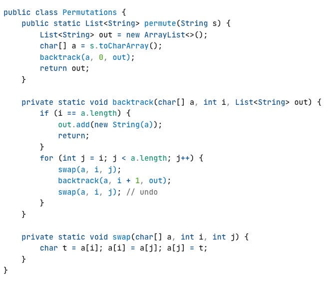
If you have a string of length 10 and try to print every permutation, that’s already several million operations and increasing n by just 1 doubles or triples the workload instantly.

These kinds of brute-force solutions are mostly used for very small inputs. Instead, we rely on smarter techniques like dynamic programming, branch and bound , or heuristics to reduce the problem space.

---

3. Space Complexity

So far, we’ve focused on time complexity, how fast an algorithm runs as input size grows.

But Big O also applies to memory usage, and that is called space complexity.

In interviews, you’ll often be asked to analyze both time and space complexity —because in real systems, performance isn’t just about speed…It’s also about how much memory your solution consumes.

Space complexity tells you how much extra memory your algorithm uses in addition to the input itself.

This extra memory can come from:

• Temporary data structures like arrays, hash maps, stacks, queues, etc.

• Recursion call stack frames

• or Intermediate buffers used during computation

Even if your algorithm is fast, it may still waste memory, which can be a serious problem in large-scale systems or environments with limited RAM.

Now, lets look at popular space complexities you will come across:

1) Constant Space - O(1)

If you scan an array to find the maximum value, you only store one variable to track the current max.

int maxValue(int[] a) {
    int max = a[0];

    for (int i = 1; i < a.length; i++) {
        if (a[i] > max) {
            max = a[i];
        }
    }

    return max;
}

So while the input size may grow, your extra space stays constant.

2) Linear Space - O(n)

Now suppose you collect all even numbers from the array into a new list.

List<Integer> collectEvens(int[] a) {
    List<Integer> evens = new ArrayList<>();

    for (int x : a) {
        if ((x & 1) == 0)
            evens.add(x);
    }

    return evens;
}

If half the numbers are even, that’s roughly n/2 elements which still counts as O(n) space.

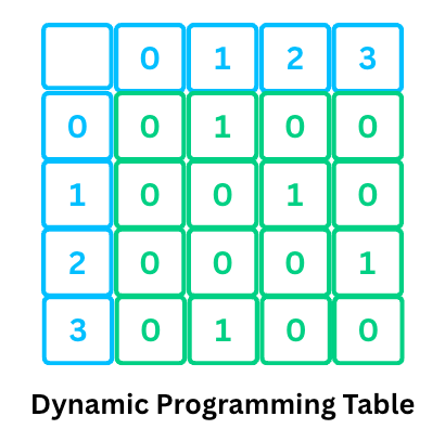
3) Quadratic Space - O(n²)

Storing a full matrix (like an adjacency matrix or Dynamic Programming (DP) table) of size n × n takes O(n²) space.

4) Space from Recursion

Space complexity isn’t only about the extra data structures you create. Recursion also consumes memory through the call stack, and this often goes unnoticed.

Every recursive call adds a new frame to the stack until the function returns. Depending on the algorithm, this stack usage can range from logarithmic to linear, or even worse.

For example, the naive recursive Fibonacci solution branches twice for each call. It takes O(2ⁿ) time but still uses O(n) space because at most n calls are active on the stack at once.

For Depth First Search (DFS) on a tree, the stack depth is proportional to the height h of the tree.

• In a balanced tree, h = O(log n) → so space is O(log n)

• In the worst case (a skewed tree), h = O(n) → so space becomes O(n)

---

4. Rules for Calculating Big O

Now, lets talk about how to actually calculate the complexity of a piece of code.

The simplest way is to break your code down into parts and analyze each part separately.

Rule 1: Add Complexities of Sequential Operations

If your algorithm performs one block of work after another, you add their time complexities.

Imagine your code has two separate, sequential loops:

// Block A: O(n)
for (int i = 0; i < m; i++) {
  // ... do O(1) work
}

// Block B: O(n^2)
for (int i = 0; i < n; i++) {
  for (int j = 0; j < n; j++) {
    // ... do O(1) work
  }
}

The total runtime is the time for Block A plus the time for Block B which comes out to be O(m) + O(n^2).

Rule 2: Multiply Complexities of Nested Operations

If you algorithm has nested loop with the outer loop running n times and the inner loop running m times, the total complexity is O(n * m).

// Block A: Outer loop runs n times -> O(n)
for (int i = 0; i < n; i++) {
  
  // Block B: Inner loop runs n times -> O(n)
  for (int j = 0; j < n; j++) {
    // ... do O(1) work
  }
}

Rule 3: Drop Constant Factors

This rule states that we can ignore any constant multipliers in a Big O expression.

When you derive a time complexity expression, you may end up with something like: O(2n + 5) or O(n² + n + 10).

Big O is not about the exact number of steps, it’s about how fast your algorithm grows with input.

Whether your algorithm takes n steps or 5n steps, both grow linearly as n increases, the constant multiplier doesn’t affect the growth trend. If you double the input, the runtime for both will (roughly) double.

So we drop constant factors:

• O(2n^2) simplifies to O(n^2)

• O(5n + 100) becomes O(n)

• O(n/3) simplifies to O(n) since 1/3 is also just a constant factor

Rule 4: Drop Lower-Order Terms

If your final expression has multiple terms, you keep only the one that grows the fastest, the dominant term, and drop the rest.

Why? Because as n becomes very large, slower-growing terms become insignificant.

Lets use the example O(n^2 + n + 100).

Imaging n = 1,000,000 (one million).

• n² which is the dominant term becomes one trillion

• while n is just one million and the constant term stays at 100

At scale, the lower-order term barely makes a dent in the overall growth. So we only keep the term that dominates.

Here are more examples:

• O(n² + n) simplifies to O(n²)

• O(n³ + 10n) becomes O(n³)

• O(n³ + n² + n) simplifies to O(n³)

---

Thank you for reading!

If you found it valuable, hit a like ❤️ and consider subscribing for more such content.

If you have any questions or suggestions, leave a comment.

---

P.S. If you’re enjoying this newsletter and want to get even more value, consider becoming a paid subscriber.

As a paid subscriber, you’ll unlock all premium articles and gain full access to all premium courses on algomaster.io.

There are group discounts, gift options, and referral bonuses available.

---

Checkout my Youtube channel for more in-depth content.

Follow me on LinkedIn, X and Medium to stay updated.

Checkout my GitHub repositories for free interview preparation resources.

I hope you have a lovely day!

See you soon,
Ashish