What is GeoHashing?

Imagine you’re building a system like Uber, Google Maps, or a nearby restaurant finder.

You need to store and query millions or even billions of location points to find what's "close" to a specific point? And you want to do it fast.

But querying latitude and longitude ranges can get messy and slow, especially at scale.

That’s where GeoHashing comes in.

In this article, we’ll explore:

• What GeoHashing is

• How it works

• Common use cases

• Limitations and trade-offs

• Practical System Design Example

---

📣 Cut Code Review Time & Bugs in Half (Sponsored)

Code reviews are critical but time-consuming. CodeRabbit acts as your AI co-pilot, providing instant Code review comments and potential impacts of every pull request.

Beyond just flagging issues, CodeRabbit provides one-click fix suggestions and lets you define custom code quality rules using AST Grep patterns, catching subtle issues that traditional static analysis tools might miss.

CodeRabbit has so far reviewed more than 10 million PRs, installed on 1 million repositories, and used by 70 thousand Open-source projects. CodeRabbit is free for all open-source repo's.

---

1. The Problem: Finding Nearby Entities Efficiently

Imagine you have a database table of restaurants, with columns for latitude and longitude. A user at (lat: 34.0523, lon: -118.2438) wants to find all restaurants within a 1km radius.

How would you write this query?

A naive approach might be a "bounding box" query:

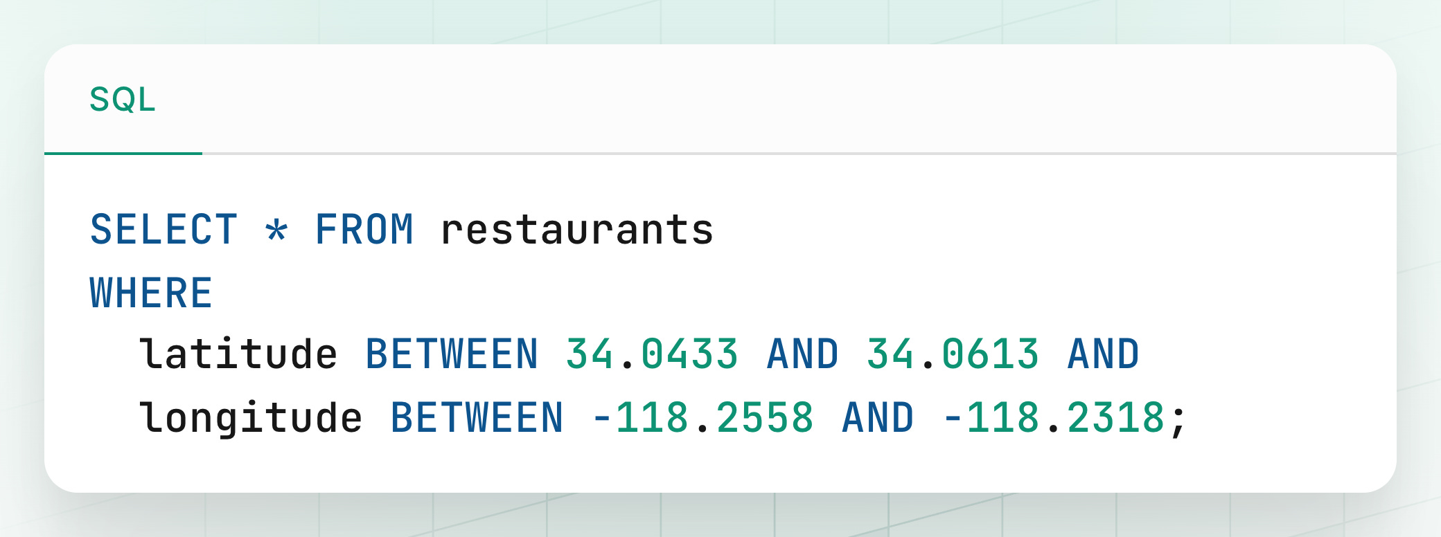
This works, but it has major performance problems at scale:

Most databases use B-tree indexes, which are fantastic for one-dimensional data. But they struggle with 2D queries. The database can use an index on latitude, but then it has to do a full scan of all matching rows to filter by longitude (or vice-versa).

A composite index on (latitude, longitude) helps, but it still doesn't truly understand spatial locality.

We need a way to represent 2D proximity in a 1D format that a standard database index can efficiently search. That’s what GeoHashing is about.

---

2. What is GeoHashing?

GeoHashing is a method of encoding geographic coordinates (latitude, longitude) into a short alphanumeric string.

It was invented by Gustavo Niemeyer in 2008 as a way to enable efficient spatial indexing and proximity search in databases and distributed systems.

Example: The coordinates for downtown San Francisco (37.7749, -122.4194) can be encoded as the geohash: 9q8yyf.

This hash looks like just a random string of characters but it has two magical properties:

1. Spatial Locality

The more characters two GeoHashes share at the beginning (i.e., the longer their common prefix), the closer those two locations are geographically.

This means: Nearby points will usually have similar GeoHash prefixes. Far-apart points will have completely different prefixes.

GeoHashes are hierarchical: each additional character in the hash zooms in to a more precise region.

Example:

• 9q8yyf and 9q9pvu share the first three characters → they belong to neighboring regions but are not immediately adjacent.

• 9q8yyf and 9q5ctr share only the first two characters → they are farther apart, likely hundreds of kilometers.

• a2sed7 → starts with a completely different prefix. It represents a geographically distant region, possibly on another continent.

2. One-Dimensional and Indexable

GeoHashes convert 2D coordinates (latitude, longitude) into a 1D string. This string can be stored in a VARCHAR or TEXT field in a relational or NoSQL database, and indexed efficiently using a B-tree or Trie.

This allows for:

• Fast lookups of nearby places

• Easy sharding based on location

• Efficient sorting and filtering using standard indexes

---

2. How GeoHashing Works?

GeoHashing may look like magic at first glance, but it’s built on a simple and elegant idea: convert a 2D geographic point into a 1D string through binary encoding and interleaving.

Let’s walk through the process of encoding a (latitude, longitude) pair into a GeoHash — step by step.

Step 1: Define the Initial Ranges

We begin by defining the global bounds of latitude and longitude:

• Latitude ranges from -90° to +90°

• Longitude ranges from -180° to +180°

These represent the full span of the Earth’s surface in both dimensions.

The goal is to gradually narrow down this range by encoding whether a coordinate lies in the lower or upper half of the current interval, similar to a binary search.

Step 2: Convert to Binary by Interleaving

Now, we start converting the latitude and longitude into binary.

Recursive Bisection

We start with the full range of values:

• Latitude: [-90°, +90°]

• Longitude: [-180°, +180°]

We then repeatedly divide each range in half and record a binary digit based on which half the coordinate falls into:

• If the value is in the lower half, we append a 0.

• If the value is in the upper half, we append a 1.

This is a lot like binary search — but instead of just narrowing down to a value, we record each decision as a bit in the final output.

Interleaving Latitude and Longitude Bits

We don’t encode latitude and longitude separately. We interleave their bits:

• 1st bit → longitude

• 2nd bit → latitude

• 3rd bit → longitude

• 4th bit → latitude
  ... and so on.

This interleaving produces a single binary string that represents the position in a Morton curve (Z-order curve), which helps preserve spatial locality.

Example:

Let’s walk through the first few steps for the point: (37.7749° N, -122.4194° W)

Step 1: Longitude → -122.4194°

Initial range: [-180°, +180°]

1. Midpoint = 0 → -122.4194 < 0 → 0 → New range: [-180, 0]

2. Midpoint = -90 → -122.4194 < -90 → 0 → New range: [-180, -90]

3. Midpoint = -135 → -122.4194 > -135 → 1 → New range: [-135, -90]

4. Midpoint = -112.5 → -122.4194 < -112.5 → 0 → New range: [-135, -112.5]

5. Midpoint = -123.75 → -122.4194 > -123.75 → 1 → New range: [-123.75, -112.5]

So first 5 longitude bits = 00101

Step 2: Latitude → 37.7749°

Initial range: [-90°, +90°]

1. Midpoint = 0 → 37.7749 > 0 → 1 → New range: [0, +90]

2. Midpoint = 45 → 37.7749 < 45 → 0 → New range: [0, 45]

3. Midpoint = 22.5 → 37.7749 > 22.5 → 1 → New range: [22.5, 45]

4. Midpoint = 33.75 → 37.7749 > 33.75 → 1 → New range: [33.75, 45]

5. Midpoint = 39.375 → 37.7749 < 39.375 → 0 → New range: [33.75, 39.375]

First 5 latitude bits = 10110

Step 3: Interleave the Bits

Interleaving the two binary sequences:

Longitude bits:  0 0 1 0 1  
Latitude bits:   1 0 1 1 0  

Interleaved:     0 1 0 0 1 1 1 0 1 0

Resulting binary string (10 bits): 0100111010

Step 4: Continue Until You Reach Desired Precision

You typically continue this process until you have:

• 30 bits → 6-character GeoHash

• 35 bits → 7-character GeoHash

• 60+ bits → very high precision

Step 3: Convert Binary to Base32 String

Once we’ve built a long binary string by interleaving latitude and longitude bits, we need to compress it into something shorter and human-readable.

This is where Base32 encoding comes in.

• Take the interleaved binary string and split it into 5-bit chunks.

• Convert each 5-bit chunk into a Base32 character.

Base32 Alphabet Used in GeoHashing:

0123456789bcdefghjkmnpqrstuvwxyz

Note: The letters a, i, l, and o are intentionally omitted to avoid confusion with similar-looking digits or letters (1, 0, etc.).

This step compresses a potentially long binary string into a short alphanumeric hash, usually between 5 to 12 characters, depending on the desired precision.

Example:

Let’s say your interleaved binary string is:

01001 11010 10011 00101

Break it into 5-bit groups and convert each chunk into a Base32 character:

• 01001 → 9

• 11010 → u

• 10011 → r

• 00101 → 5

Final GeoHash: 9ur5

Precision vs. Length

Each additional character in the GeoHash increases the precision of the location.

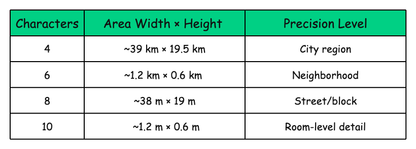
You can control the granularity of your spatial encoding just by adjusting the number.

---

3. Why Use GeoHashing?

GeoHashing offers benefits that are highly valuable in location-based services:

Efficient Proximity Search

Instead of range queries on lat/lon, you can:

• Use GeoHash prefix matching

• Search within a bounding box by comparing string prefixes

Indexing in Databases

Databases like PostgreSQL, Cassandra, and MongoDB can:

• Index strings faster than floating-point pairs

• Use trie or B-tree-based lookups for prefix search

Spatial Sharding

GeoHashes are great for sharding data in distributed systems:

• Assign prefixes to different servers/partitions

• Keep nearby data close together

---

4. Real-World Applications

GeoHashing is widely used in location-based apps and geospatial databases.

Here are some real-world examples where GeoHashing shines:

Ridesharing Platforms (e.g., Uber, Lyft)

GeoHashes can be used to group drivers and riders into spatial buckets based on their current location.

• When a rider requests a trip, the system calculates their GeoHash (e.g., to 6 or 7 characters).

• It then quickly finds drivers in the same or neighboring GeoHash cells, drastically reducing the search space.

• This enables real-time proximity matching without scanning all active drivers.

Food Delivery Services (e.g., Swiggy, Zomato)

When a user opens the app to browse nearby restaurants:

• Their coordinates are converted into a GeoHash.

• The backend queries all restaurants whose stored GeoHashes match that prefix or its neighbors.

• This allows the system to serve relevant results instantly, even with millions of entries in the database.

Geospatial Databases (e.g., Elasticsearch, MongoDB)

GeoHashing is often used under the hood in spatial indexing strategies.

• Elasticsearch supports geohash_grid aggregations to efficiently bucket documents by location.

• MongoDB can store GeoHashes for fast, prefix-based querying on 2D location fields.

---

5. Limitations and Trade-offs

GeoHashing is a powerful tool for spatial indexing but like any abstraction, it comes with trade-offs.

Advantages

• Simplicity: It maps a 2D problem to a 1D problem, allowing for extremely fast prefix searches on standard database indexes.

• Hierarchical: You can easily "zoom in" or "zoom out" by simply adjusting the length of the geohash string you use for querying. This is great for map UIs.

• Scalable: It scales horizontally very well. The workload is easily distributable.

• Database Agnostic: It works with any database that supports string indexing (PostgreSQL, MySQL, etc.).

Disadvantages

• The Edge Case Problem: You must query neighboring cells to avoid missing nearby points that fall across a boundary. This adds a little complexity to the query logic.

• Cell Shape Distortion: Geohash cells are rectangular, and their shape distorts and becomes less square-like as you move away from the equator. This means a geohash doesn't represent a uniform circular area.

• False Positives: Two points can be in the same geohash cell but at opposite corners, making them farther apart than a point in a neighboring cell. This is why the final, precise distance calculation is necessary.

• Not a True k-NN: On its own, geohashing is a proximity search, not a true "k-Nearest Neighbors" search. You must combine it with a post-filtering distance calculation to get accurate k-NN results.

---

6. Using GeoHashing in a System Design

Now let’s look at how to practically implement GeoHashing to build a location-based feature like showing nearby restaurants.

1. Indexing the Data

Let's say we have a restaurants table in our database.

To enable fast geospatial queries:

• We add a new column called geohash.

• Every time a restaurant is created or its location is updated, we:

  • Calculate its GeoHash (e.g., with 7-character precision).

  • Store it in the geohash column.

This prepares the data for efficient prefix-based lookups.

Schema Example:

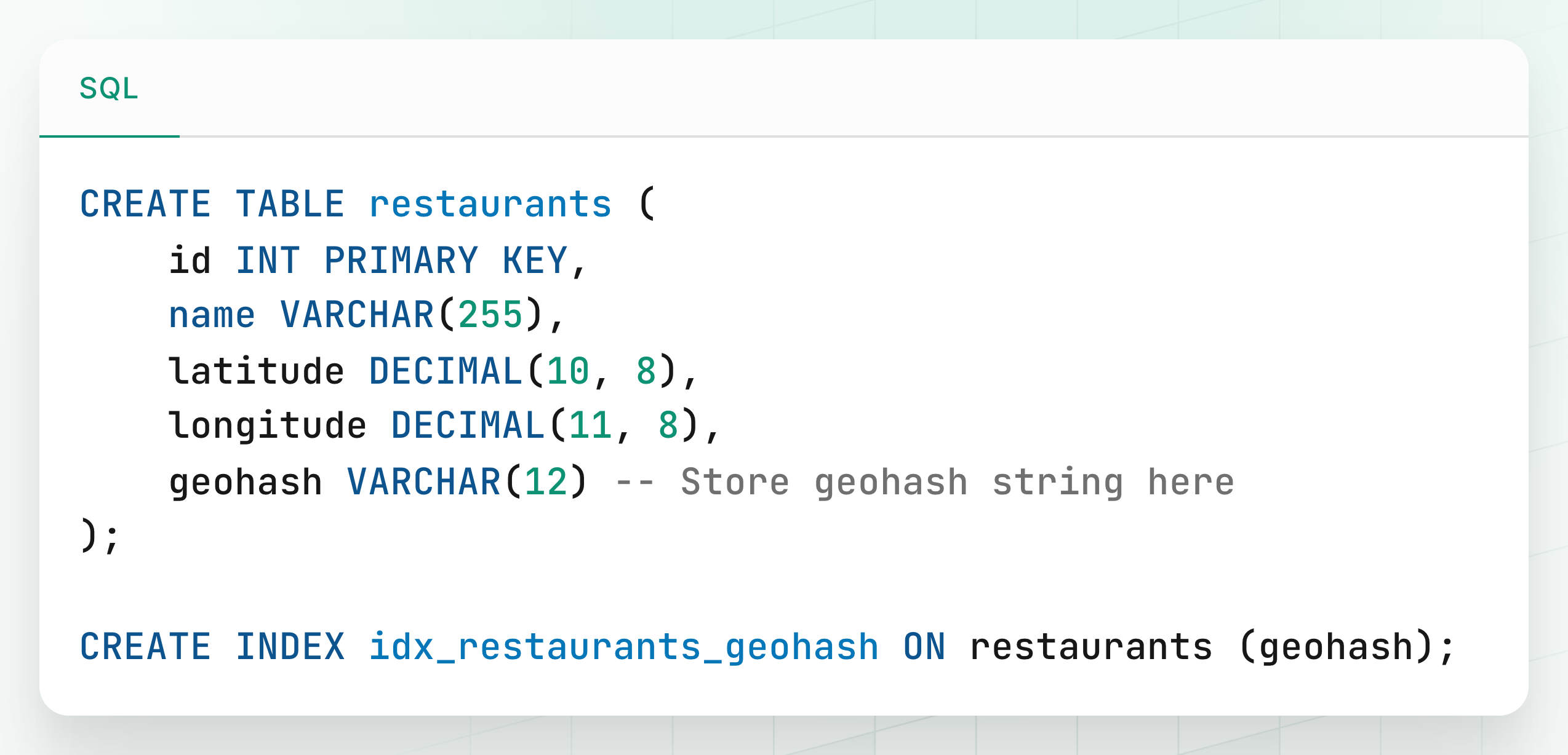
Since GeoHash is stored as a string, we can index it with a B-tree which enables fast, lexicographical prefix filtering.

2. Querying for Nearby Items

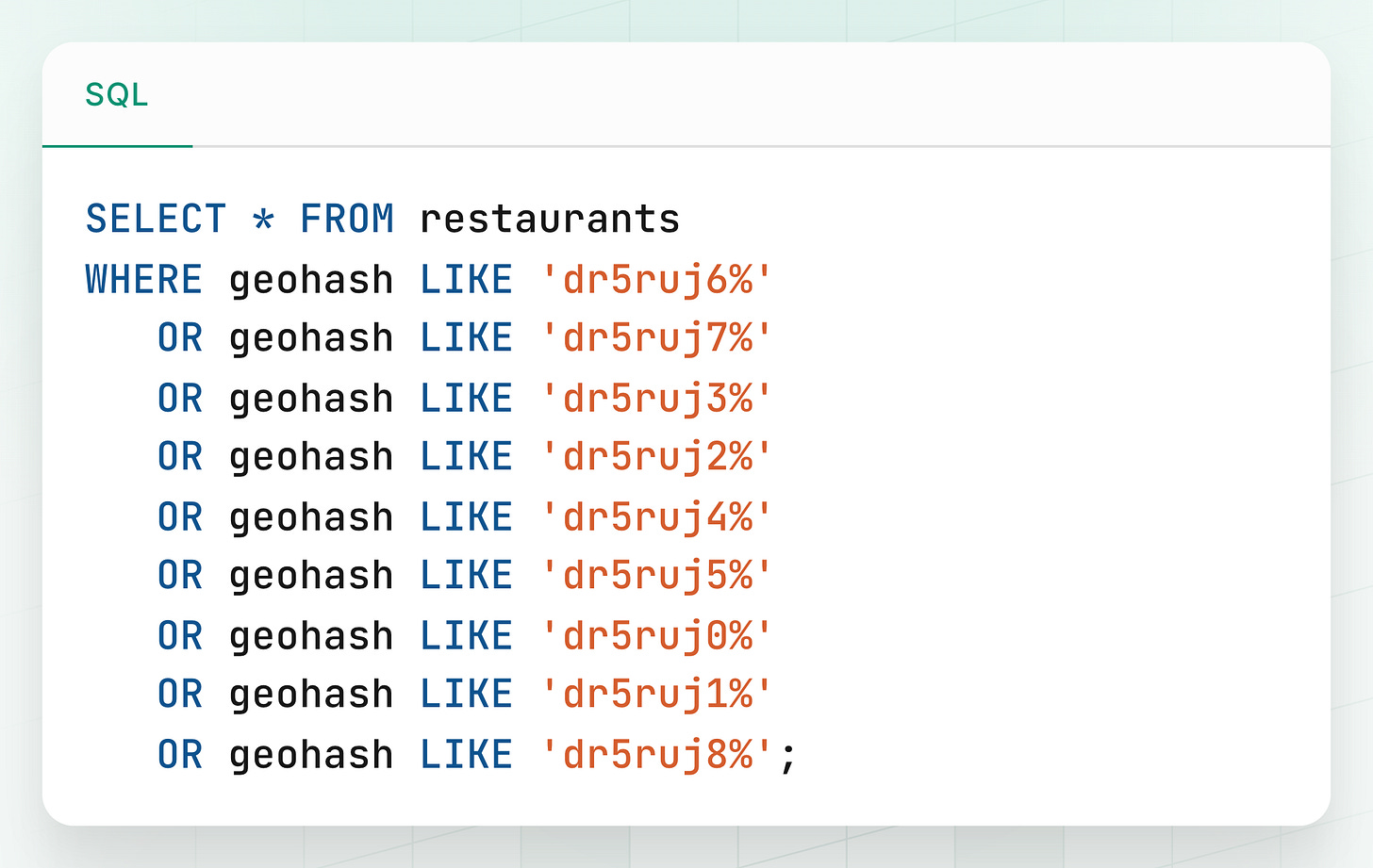
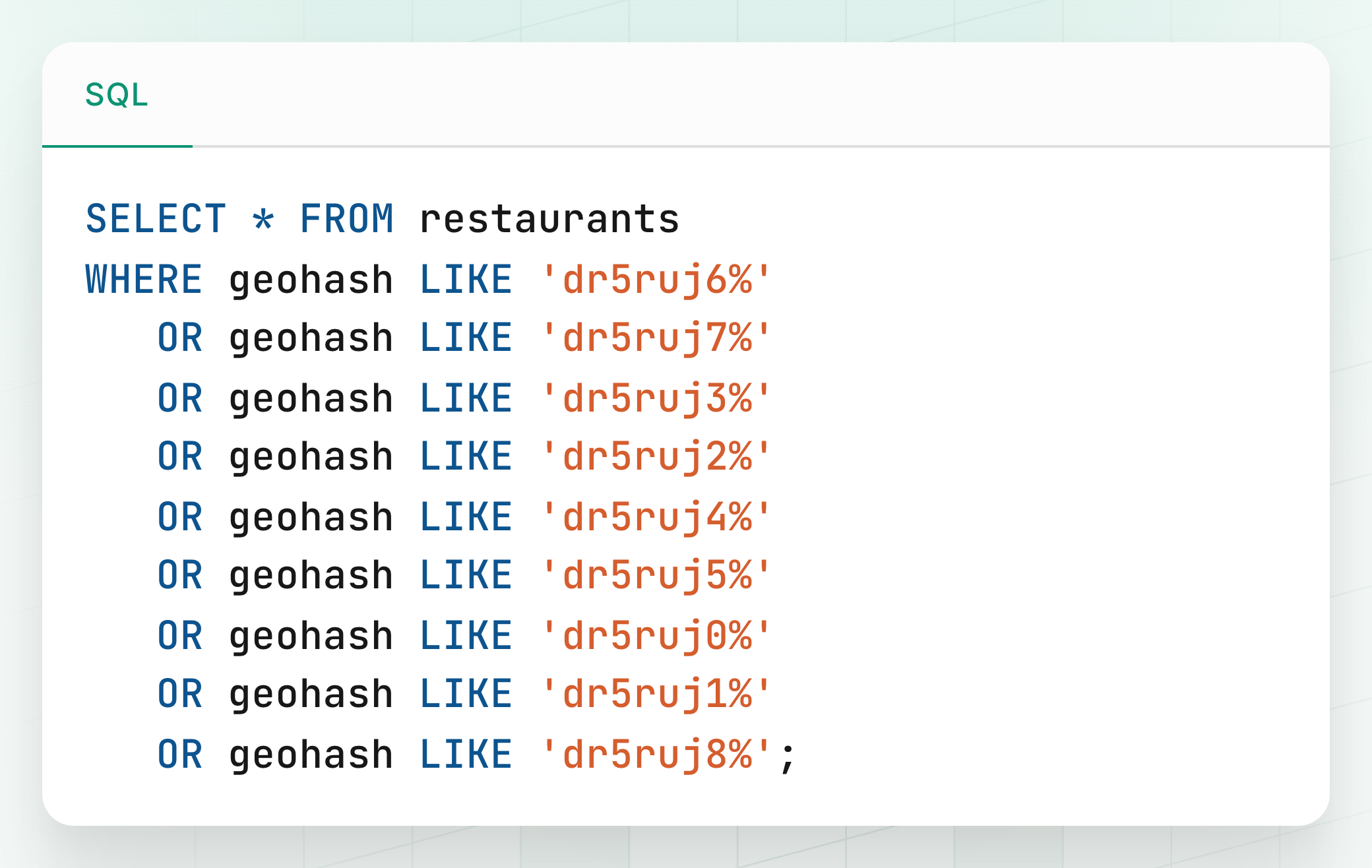
Let's say a user is at a location that maps to GeoHash: dr5ruj6.

To find nearby restaurants within, say, a 200-meter radius, the most basic query would be:

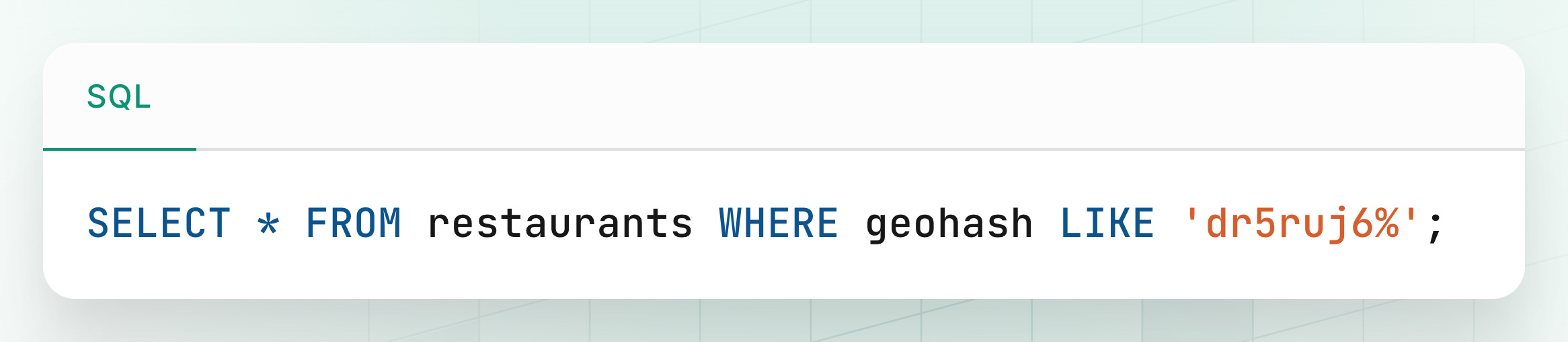
This works well in many cases, but there's a critical flaw.

The Edge Case Problem

What if the user is standing right on the edge of the dr5ruj6 cell, and the closest restaurant is just across the boundary in a neighboring cell like dr5ruj7?

The query above would miss that restaurant even though it may be just 20 meters away.

3. The Solution: Include Neighboring Cells

Each GeoHash defines a bounding box. If we also consider the 8 immediate neighbors around that box, we cover the full surrounding area, eliminating blind spots at cell edges.

Full Query Strategy:

1. Get User Location: Capture user's current latitude and longitude.

2. Calculate Base Geohash: Convert that location to a GeoHash with your chosen precision (e.g., dr5ruj6).

3. Calculate Neighbors: Use a GeoHash utility/library to get the 8 surrounding GeoHashes.

4. Query all 9 cells: Query the database for items whose geohash starts with any of these 9 prefixes (the user's cell + 8 neighbors).

   

4. Post-Filtering

The GeoHash-based prefix query is fast, but still slightly approximate.

So once we get the candidate set of restaurants, we do a second, more precise filtering step:

• Use the Haversine formula or Vincenty formula to compute the exact distance between the user’s location and each candidate.

• Filter out any restaurants that fall outside the desired radius (e.g., beyond 200m).

• Sort the remaining results by distance to return the nearest ones first.

The expensive Haversine computation is done on hundreds of rows, not millions, which keeps the system performant.

---

7. Alternatives to GeoHashing

While GeoHashing is a fast, lightweight, and scalable approach to spatial indexing, it's not the only option.

Several other data structures are commonly used in geospatial systems, each with their own strengths and trade-offs:

Quadtrees / K-d Trees

These are tree-based spatial partitioning structures that recursively divide the space into smaller regions.

• Quadtrees divide 2D space into four quadrants at each level.

• K-d Trees divide k-dimensional space by alternating splitting axes (e.g., latitude and longitude).

GeoHashing can be conceptually seen as a simplified, linearized representation of a quadtree traversal, following a space-filling curve like a Z-order (Morton) curve.

R-trees

R-trees are commonly used in spatial databases such as PostGIS (PostgreSQL extension), Oracle Spatial, and SQLite’s SpatiaLite.

• They group nearby objects into bounding rectangles.

• Each node in the tree contains the minimum bounding rectangle (MBR) that encloses its children.

• This structure supports efficient queries for containment, intersection, and nearest neighbors.

---

Thank you for reading!

If you found it valuable, hit a like ❤️ and consider subscribing for more such content.

If you have any questions or suggestions, leave a comment.

---

P.S. If you’re enjoying this newsletter and want to get even more value, consider becoming a paid subscriber.

As a paid subscriber, you'll get full access to all premium articles and access to all courses at algomaster.io

There are group discounts, gift options, and referral bonuses available.

---

Checkout my Youtube channel for more in-depth content.

Follow me on LinkedIn, X and Medium to stay updated.

Checkout my GitHub repositories for free interview preparation resources.

I hope you have a lovely day!

See you soon,
Ashish