

How Load Balancers Actually Work
A Deep Dive

A load balancer is one of the most foundational building blocks in distributed systems. It sits between clients and your backend servers and spreads incoming traffic across a pool of machines, so no single server becomes the bottleneck (or the single point of failure).
But the interesting questions start after the definition:
How does the load balancer decide which server should handle a request?
What’s the difference between L4 and L7 Load Balancers?
What happens when a server slows down or goes offline mid-traffic?
How can the load balancer ensure that request from the same client always go to the same server?
And what happens if the load balancer itself goes down?
In this article, we’ll answer these questions and build an intuitive understanding of how load balancers work in real systems.
Let’s start with the basics: why we need load balancers in the first place.
1. Why Do We Need Load Balancers?
Imagine a web app with just one server. Every user request hits the same machine.
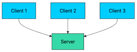
It works… until it doesn’t. This “single-server” setup has a few fundamental problems:
Single Point of Failure: If the server crashes, your entire application goes down.
Limited Scalability: A single server can only handle so many requests before it becomes overloaded.
Poor Performance: As traffic increases, response times degrade for all users.
No Redundancy: Hardware failures, software bugs, or maintenance windows cause complete outages.
A load balancer solves these problems by distributing traffic across multiple servers.
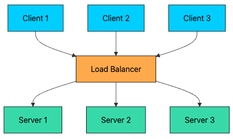
With this setup, you get:
High Availability: If one server fails, traffic is automatically routed to healthy servers.
Horizontal Scalability: You can add more servers to handle increased load.
Better Performance: Requests are distributed, so no single server is overwhelmed.
Zero-Downtime Deployments: You can take servers out of rotation for maintenance without affecting users.
But how does the load balancer decide which server should handle each request?
2. Load Balancing Algorithms
The load balancer uses algorithms to distribute incoming requests. Each algorithm has different characteristics and is suited for different scenarios.
Below are the most common ones you’ll see in real systems.
2.1 Round Robin
The simplest algorithm. Requests are distributed to servers in sequential order.
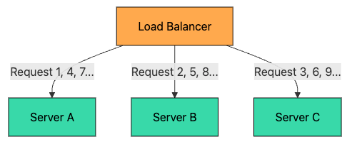
Request 1 → Server A
Request 2 → Server B
Request 3 → Server C
Request 4 → Server A  (cycle repeats)
Request 5 → Server B
...
Pros:
Simple to implement
Works well when all servers have equal capacity
Predictable distribution
Cons:
Does not account for server load or capacity differences
A slow request on one server does not affect the distribution
Best for: Homogeneous server environments where all servers have similar specs and requests have similar processing times.
2.2 Weighted Round Robin
An extension of Round Robin where servers are assigned weights based on their capacity.
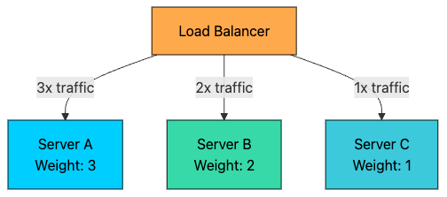
Server A (weight=3): Handles 3 out of every 6 requests
Server B (weight=2): Handles 2 out of every 6 requests
Server C (weight=1): Handles 1 out of every 6 requests
Pros:
Still simple
Better for mixed instance sizes (e.g., 2 vCPU + 4 vCPU + 8 vCPU)
Cons:
Still not load-aware in real time
If one server becomes slow (GC pause, noisy neighbor, warm cache vs cold cache), it will still get its scheduled share
Best for: Heterogeneous environments where servers have different capacities (e.g., different CPU, memory, or network bandwidth).
2.3 Least Connections
Routes requests to the server with the fewest active connections.
This algorithm is dynamic, it considers the current state of each server rather than using a fixed rotation.
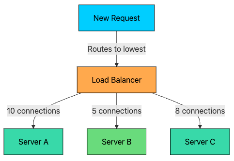
Server A: 10 active connections
Server B: 5 active connections  ← Next request goes here
Server C: 8 active connections
Pros:
Adapts to varying request processing times
Naturally balances load when some requests take longer than others
Cons:
Requires tracking connection counts for each server
Slightly more overhead than Round Robin
Best for: Applications where request processing times vary significantly (e.g., database queries, file uploads).
2.4 Weighted Least Connections
Combines Least Connections with server weights. The algorithm considers both the number of active connections and the server’s capacity.
Score = Active Connections / Weight

Server A: 10 connections, weight 5 → Score = 2.0
Server B: 6 connections, weight 2  → Score = 3.0
Server C: 4 connections, weight 1  → Score = 4.0

Next request goes to Server A (lowest score)
Pros:
Works well for mixed instance sizes and mixed request durations
More robust than either “weighted” or “least connections” alone
Cons:
Needs reliable tracking + weight tuning
Still uses connections as a proxy for load (not always perfect)
Best for: Heterogeneous environments with varying request processing times.
2.5 IP Hash
The client’s IP address is hashed to determine which server handles the request. The same client IP always goes to the same server.
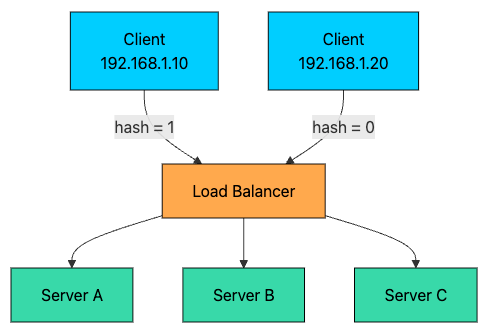
hash(192.168.1.10) % 3 = 1 → Server B
hash(192.168.1.20) % 3 = 0 → Server A
hash(192.168.1.30) % 3 = 2 → Server C
Pros:
Simple session persistence without cookies
No additional state to track
Cons:
Uneven distribution if IP addresses are not uniformly distributed
Server additions/removals cause redistribution of clients
Best for: Applications requiring basic session persistence without cookie support.
2.6 Least Response Time
Routes requests to the server with the fastest response time and fewest active connections.
The load balancer continuously measures:
Average response time for each server
Number of active connections
Pros
Optimizes for perceived performance
Can avoid slow/unhealthy servers before they fully fail
Cons
Highest operational complexity (needs continuous measurement and smoothing)
Can “overreact” to noise without careful tuning (feedback loops)
Requires good metrics and stable observation windows
Best for: Latency-sensitive applications where response time is critical.