

Neural Networks Explained In Plain English


Welcome to another edition of the AI Engineering series, where we cover important AI/ML concepts and how to build modern AI applications.
This is a guest post by Dr. Ashish Bamania. He’s an AI engineer and author of multiple newsletters including Into AI and Into Quantum.
All popular AI systems that you see today are made up of basic computing units called Neurons or Perceptrons. These connect to form a network called a Neural network that performs various complex computations.
In this lesson, we will understand how neural networks work and how they solve challenging problems, such as generating text, recognizing objects, controlling a robot, and more.
Let’s begin!
To Begin, What is a Neuron?
A Neuron (also called a Perceptron) is inspired by a nerve cell (also called a Neuron) in the body.
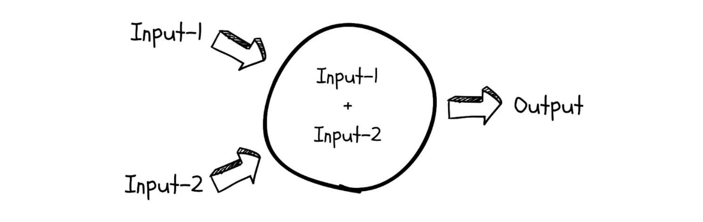
It accepts single or multiple inputs, performs calculations on them, and generates an output.
It is implemented using a simple linear equation as shown below.
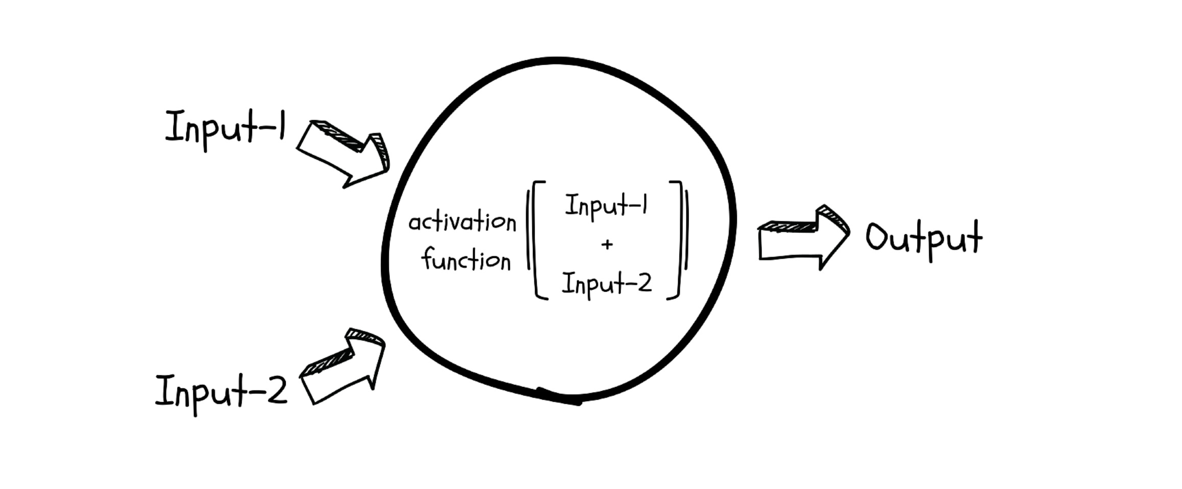
The job of a neuron is to find or approximate a function that somehow connects the output to its inputs. This function can be as simple or complex as possible.
Now that’s tough, especially when a neuron is just a linear function. Since most real-world functions cannot be approximated with a linear function, a neuron uses an Activation function to capture the non-linearities in its input.
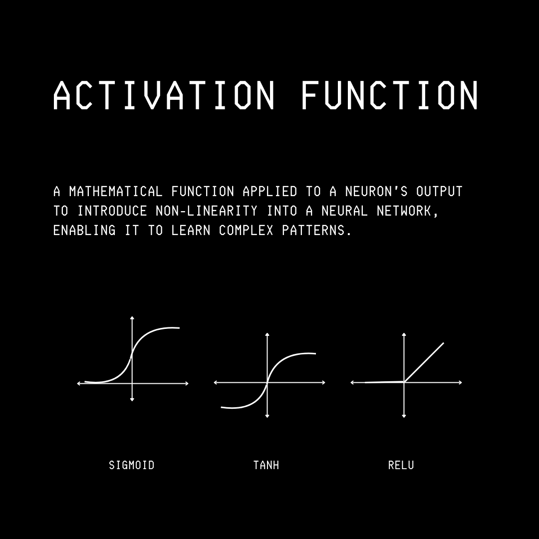
Some of the commonly used Activation functions in neural networks are as follows:
Sigmoid: An S-shaped function that squashes an input into a value between 0 and 1.
TanH: An S-shaped function that squashes an input into a value between -1 and 1.
ReLU or Rectified linear unit: A function that outputs the input directly if it is positive, but converts all negative inputs into 0.
How does a Neuron learn?
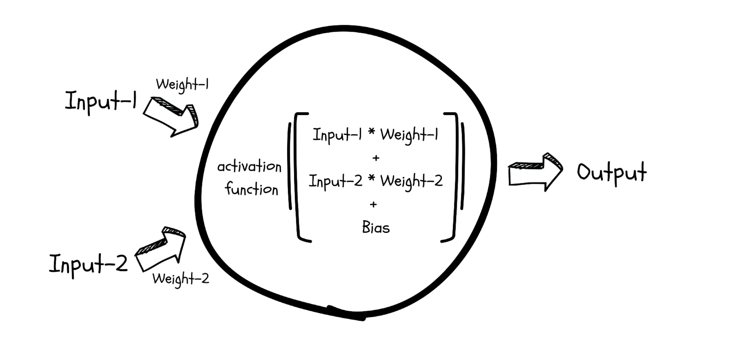
A neuron uses parameters called Weights and Biases to learn the relationship between its inputs and outputs. These parameters are not fixed and change as a neuron learns.
A neuron on its own isn’t a very powerful learner, and this is why multiple neurons are stacked together to form a Neural network. Since neurons are also called Perceptrons and these networks consist of multiple layers of them, this architecture is also called a Multi-layer Perceptron (MLP).
Stacking neurons into a network
Check out an example below where we have stacked 5 neurons together in 3 layers.
Since the output of each neuron is transmitted to every other neuron in the next layer, these are called Dense layers. (The other category being Sparse layers, which we won’t discuss in this article.)
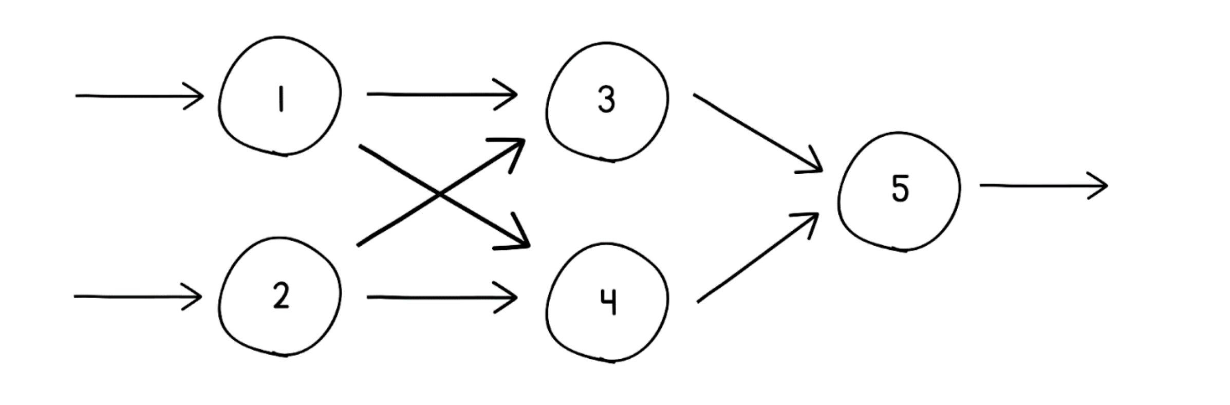
The layers of the neural network are categorized as follows:
Input layer (with neurons 1 and 2): Takes an input
Hidden layer (with neurons 3 and 4): Performs most calculations
Output layer (with neuron 5): Outputs the result
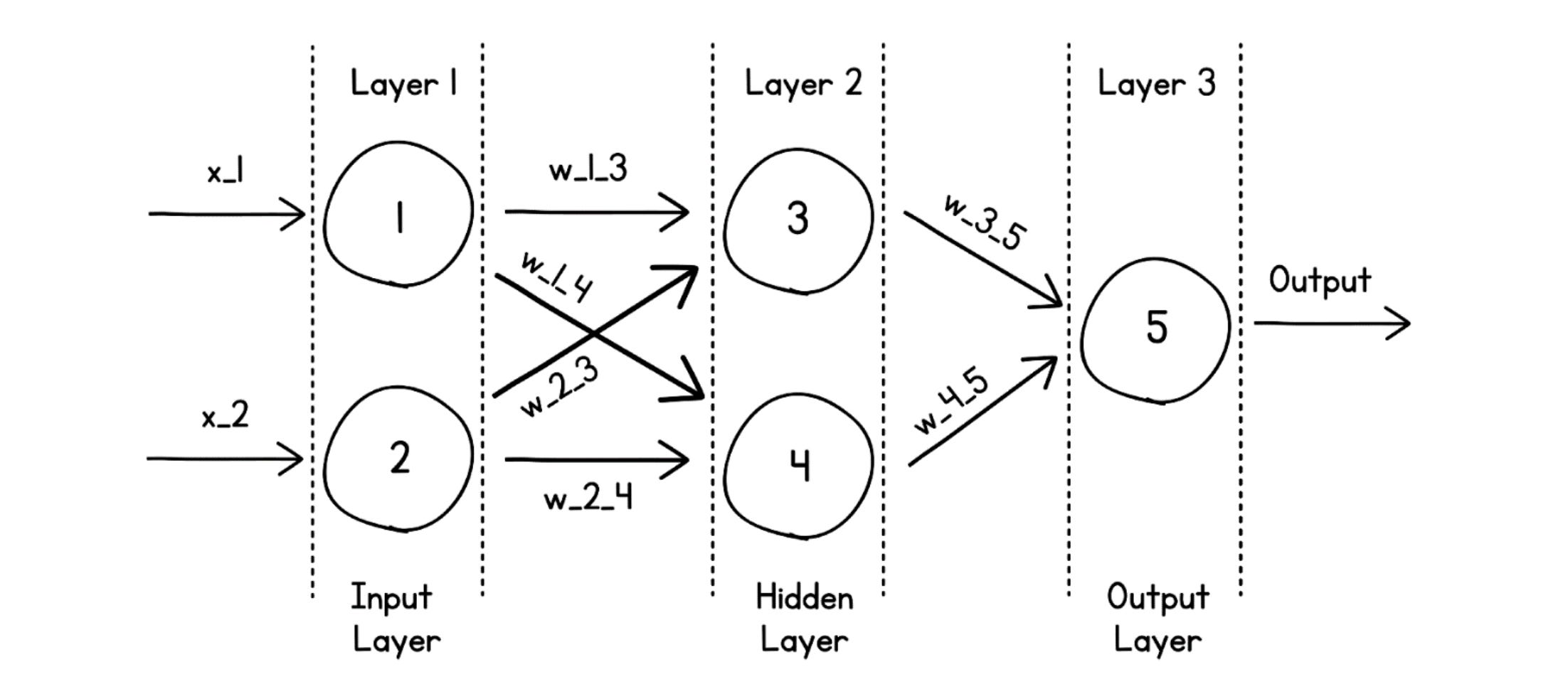
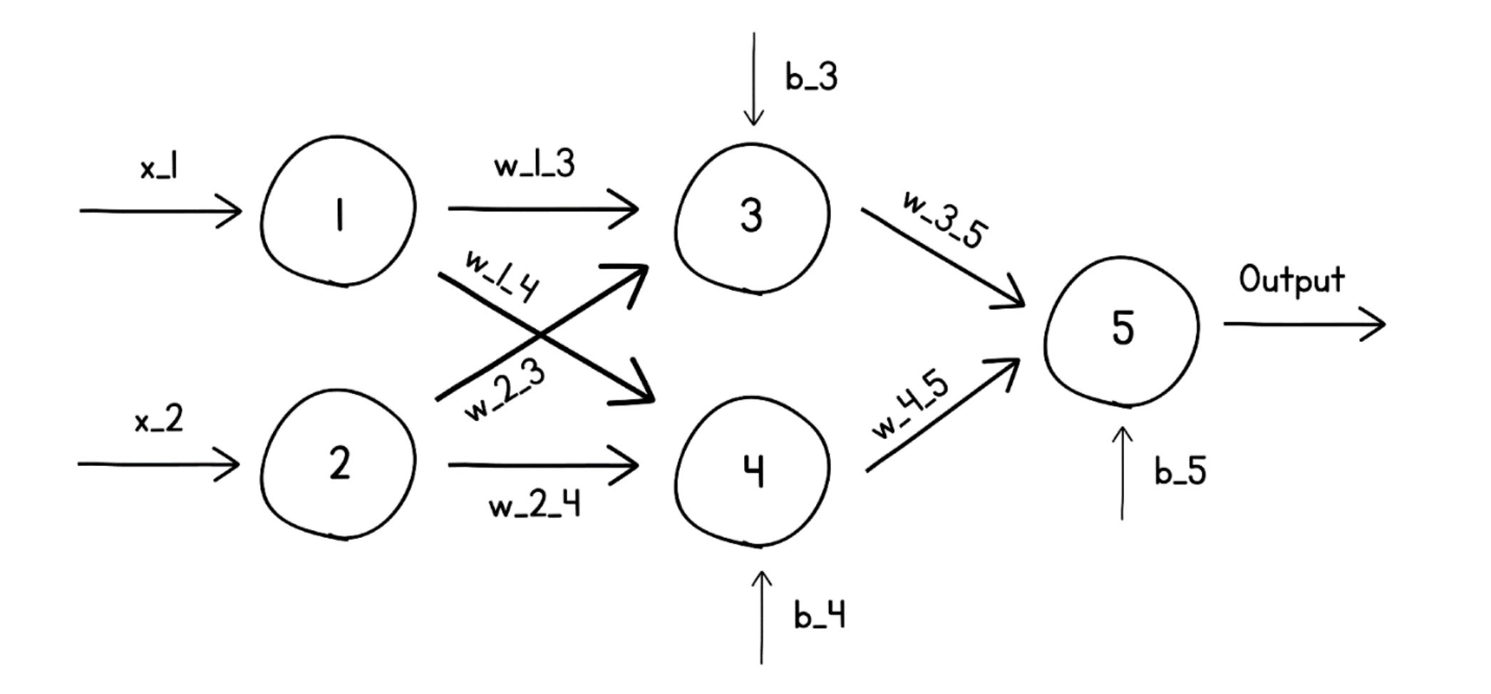
Zooming in, each neuron in these layers receives input, which is multiplied by a unique weight and bias terms specific to that neuron, and generates an output that is passed to another neuron.
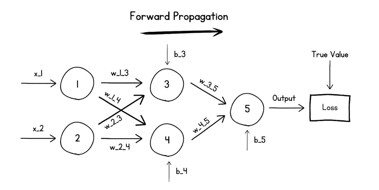
These calculations continue till a final output from the neural network is generated. This process of calculating the output of a neural network from its inputs is called the Forward Pass, or Forward Propagation.
Since data flows from the Input layer to the Output layer, which is an imagined forward direction, this network is called a Feed-Forward Network. (The other category being Recurrent neural networks, which we won’t be discussing in this article.)
How does a neural network learn?
A neural network learns by iteratively updating its parameters until it approximates the function that maps its inputs to outputs.
At the beginning of training, when a neural network generates an output given its inputs, the output is mostly gibberish because the parameters in each neuron are randomly set.
For learning, the generated output is compared with the true value (the output that we intend the neural network to generate) using a Loss function.
This loss function is a mathematical formula that measures the error between the network’s generated/predicted output and the true value.
Some commonly used loss functions are:
Mean Absolute Error: The average of the absolute differences between the network’s output values and the true values (used for regression problems)
Mean Squared Error: The average squared difference between the network’s output values and the true values (used for regression problems)
Binary/ Categorical Cross-Entropy: Measure of the performance of a classification model whose output is a probability value between 0 and 1.
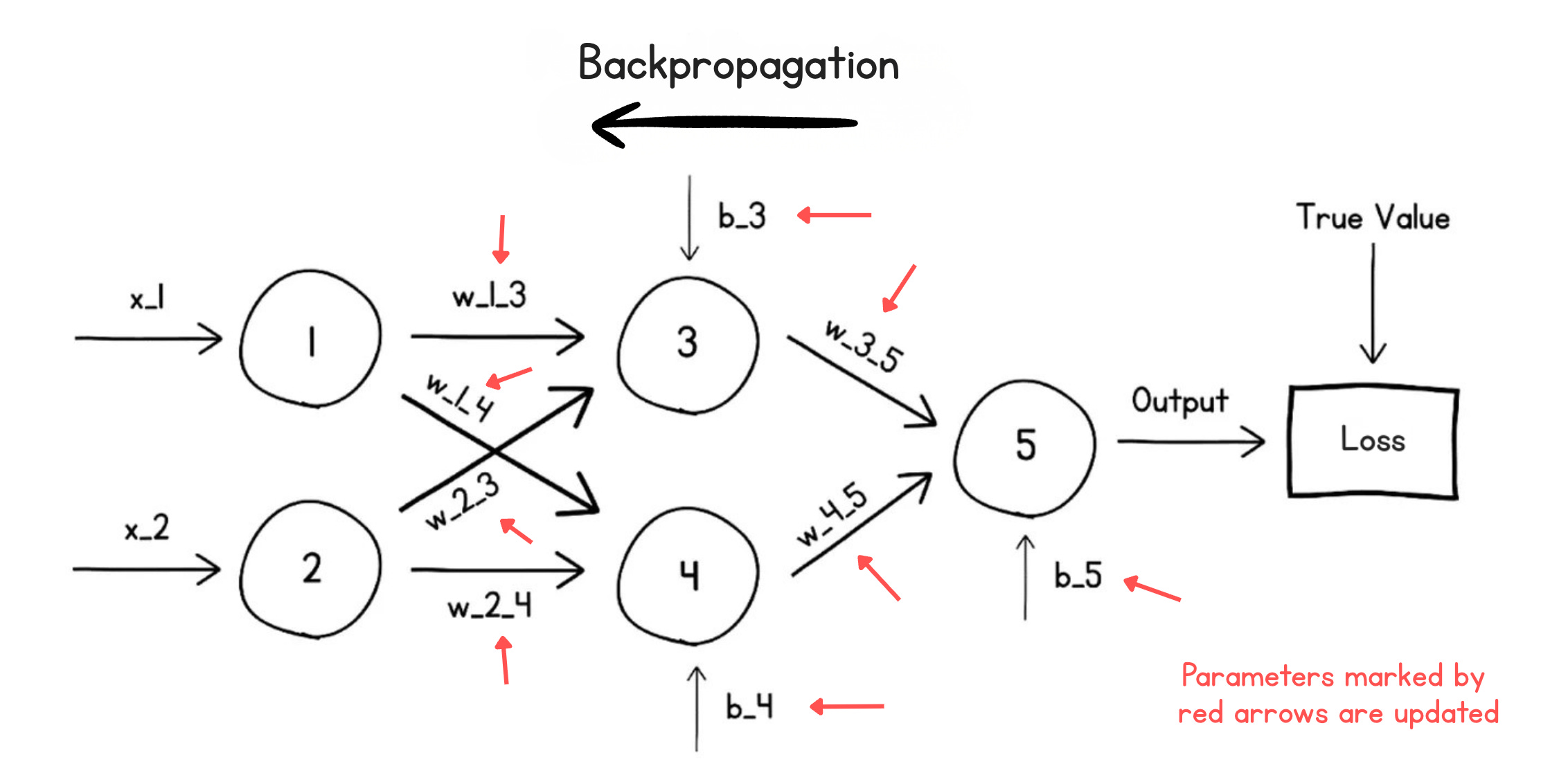
This measure of error or Loss is used to update the parameters (weights and biases) in a process called the Backward Pass or Backpropagation.
Each parameter is updated in proportion to its contribution to the overall loss. This ensures that, in the next forward pass, the loss is smaller than in this one, and the model learns by reducing the loss.
The algorithm used for this parameter update process is called an Optimization algorithm, or Optimizer. Some commonly used optimizers are as follows:
To ensure that parameter values do not change a lot in a single step of optimization, updates are scaled using a value called the Learning rate.
These training runs, each consisting of a forward and a backward pass, continue for multiple turns.
The loss value decreases in each run until the network starts outputting a value that is very close to the true value. This finishes the neural network training.
An example of a neural network learning to identify images
Let’s take an example of a neural network learning to identify whether a given image is of a cat or a dog.
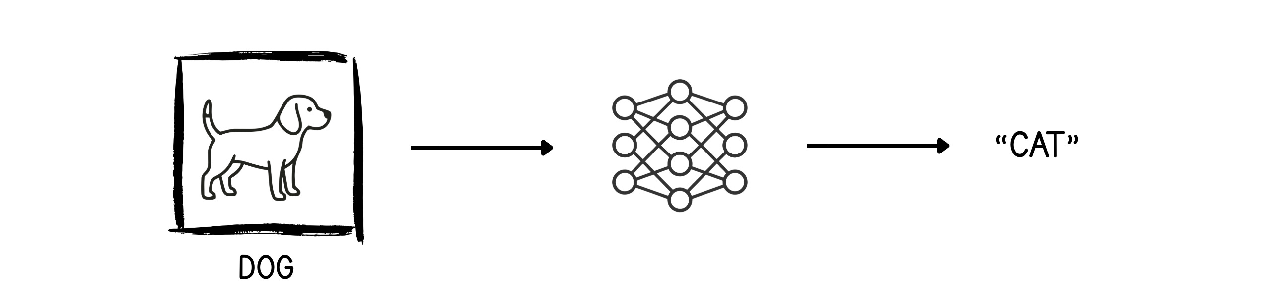
The training starts with a huge dataset of mixed images of dogs and cats. At each step, the network is given an image as input and asked to output what it thinks the image is (Forward pass).
In the following example, the untrained neural network outputs “Cat” for the dog’s image. We need to fix this.
The output (“Cat”) and the true value (“Dog”) are compared using a Loss function, which outputs an error called Loss.
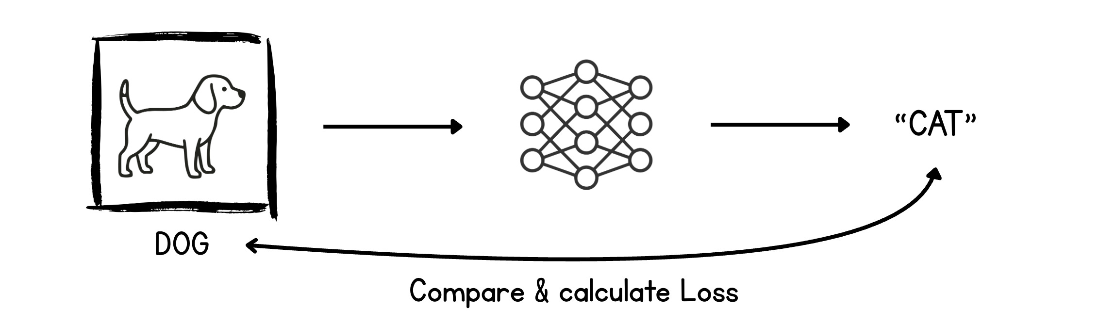
This loss value is then used to update the parameters during the backward pass. The parameter update is in a direction that leads to lower loss in the next training run.
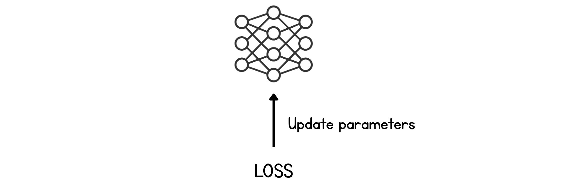
This process continues until the neural network generates the correct output (“Dog”) for the image.
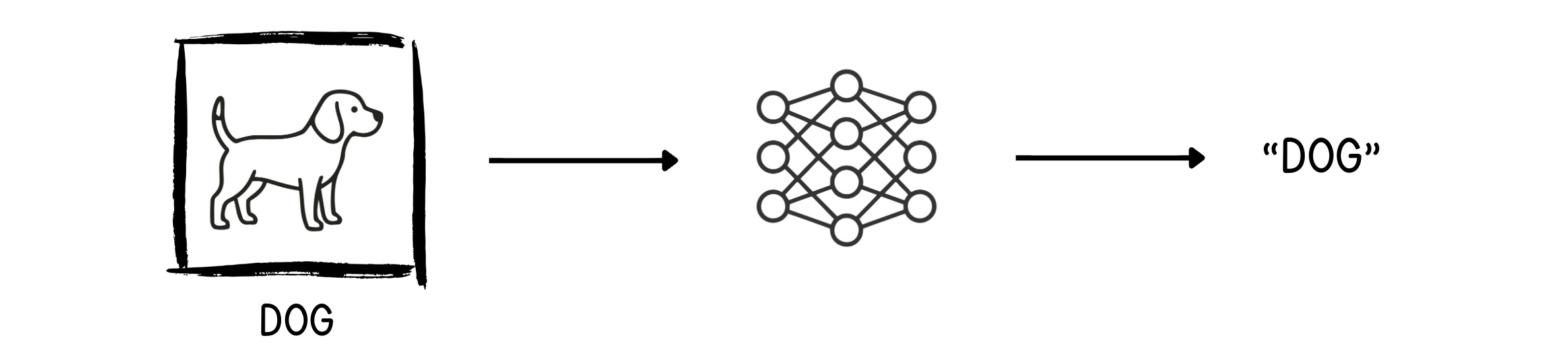
I’ve only shown this for dog images, but a similar process applies to cat images as well. The training ends when the neural network starts identifying the correct label for the images.
 | A guest post by
|
Very well written! Made me think about how often people jump to using tools without understanding what’s happening underneath. How do you approach deciding the number of layers and neurons in a neural network for a new problem, especially when there isn’t a clear reference point or prior work to guide the architecture?
This is the most concise and easy explanation on neural network training.
Though I have some questions.